Analyzing forest change with gfcanalysis

Overview

This gfcanalysis R package facilitates simple analyses using the Hansen et al. 2013¹ Global Forest Change dataset. The package was written to analyze forest change in within the Zone of Interaction surrounding each of the forest monitoring sites of the Tropical Ecology Assessment and Monitoring (TEAM) Network.

If you need help with any of the functions in the package, see the help files for more information. For example, type ?download_tiles in R to see the help file for the download_tiles function.

Getting started

This post will outline an analysis using the gfcanalysis package. Note that as the computations are intensive, some parts of this analysis may take some time to run (about 30 minutes total to run all of the code outlined here). If you do not already have the GFC product data downloaded on your computer, downloading the dataset will also take some time (though this process is automated by gfcanalysis).

To get started, first install the gfcanalysis package from CRAN. Also install the rgdal package needed for reading/writing shapefiles if you do not already have it.

if (!require(gfcanalysis)) install.packages('gfcanalysis')

## Loading required package: gfcanalysis
## Loading required package: raster
## Loading required package: sp

if (!require(rgdal)) install.packages('rgdal')

## Loading required package: rgdal
## rgdal: version: 0.8-16, (SVN revision 498)
## Geospatial Data Abstraction Library extensions to R successfully loaded
## Loaded GDAL runtime: GDAL 1.10.1, released 2013/08/26
## Path to GDAL shared files: C:/Users/azvoleff/R/win-library/3.2/rgdal/gdal
## GDAL does not use iconv for recoding strings.
## Loaded PROJ.4 runtime: Rel. 4.8.0, 6 March 2012, [PJ_VERSION: 480]
## Path to PROJ.4 shared files: C:/Users/azvoleff/R/win-library/3.2/rgdal/proj

Indicate where we want to save GFC tiles downloaded from Google. For any given AOI, the script will first check to see if these tiles are available locally (in the below folder) before downloading them from the server - so I recommend storing ALL of your GFC tiles in the same folder. For this example we will use “.” - the current working directory of the R session.

output_folder <- "."

Set the threshold for forest/non-forest based on the treecover2000 layer in the GFC product:

forest_threshold <- 90

Downloading data from Google server for a given AOI

Load an area of interest. For this example we use a shapefile of the Zone of Interaction (ZOI) of the TEAM Network site in Nam Kading National Protected Area, Laos. Notice that first we specify the folder the shapefile is in (here it is a “.” indicating the current working directory), and then the name of the shapefile without the “.shp”. To follow along with this example, download this shapefile of the ZOI.

aoi <- readOGR('.', 'ZOI_NAK_2012_EEsimple')

## OGR data source with driver: ESRI Shapefile 
## Source: ".", layer: "ZOI_NAK_2012_EEsimple"
## with 1 features and 3 fields
## Feature type: wkbPolygon with 2 dimensions

Calculate the tiles needed to cover the AOI:

tiles <- calc_gfc_tiles(aoi)
print(length(tiles)) # Number of tiles needed to cover AOI

## [1] 1

To check the overlap between the tiles and the aoi, you can make a plot of the needed tiles and the AOI using R’s plotting functions:

plot(tiles)
plot(aoi, add=TRUE, lty=2, col="#00ff0050")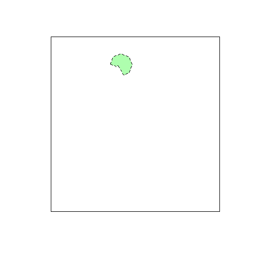

center

Now, check to see if these tiles are already present locally, and download them if they are not. By default the “first” and “last” composite surface reflectance images are not downloaded. To also download these images specify first_and_last=TRUE.

download_tiles(tiles, output_folder, first_and_last=FALSE)

## 1 tiles to download/check.
## 0 file(s) succeeded, 5 file(s) skipped, 0 file(s) failed.

Performing thresholding and calculating basic statistics

Extract the GFC data for this AOI from the downloaded GFC tiles, mosaicing multiple tiles as necessary (if needed to cover the AOI). Save this extract in GeoTiff format in the current working directory (can also save as ENVI format, Erdas format, etc.)

gfc_extract <- extract_gfc(aoi, output_folder, filename="NAK_GFC_extract.tif")

The extracted dataset has 5 layers (not yet thresholded):

gfc_extract

## class       : RasterBrick 
## dimensions  : 4358, 4761, 20748438, 5  (nrow, ncol, ncell, nlayers)
## resolution  : 0.0002778, 0.0002778  (x, y)
## extent      : 103.5, 104.8, 17.83, 19.04  (xmin, xmax, ymin, ymax)
## coord. ref. : +proj=longlat +datum=WGS84 +no_defs +ellps=WGS84 +towgs84=0,0,0 
## data source : C:\Users\azvoleff\Code\Misc\azvoleff.github.io\Rmd\2014-03-25-analyzing-forest-change-with-gfcanalysis\NAK_GFC_extract.tif 
## names       : treecover2000, loss, gain, lossyear, datamask 
## min values  :             0,    0,    0,        0,        1 
## max values  :           100,    1,    1,       12,        2

Threshold the GFC data based on a specified percent cover threshold (0-100), and save the thresholded layers to a GeoTiff:

gfc_thresholded <- threshold_gfc(gfc_extract, forest_threshold=forest_threshold, 
                                 filename="NAK_GFC_extract_thresholded.tif")

Coding of the thresholded output

The thresholded dataset has 5 layers:

gfc_thresholded

## class       : RasterBrick 
## dimensions  : 4358, 4761, 20748438, 5  (nrow, ncol, ncell, nlayers)
## resolution  : 0.0002778, 0.0002778  (x, y)
## extent      : 103.5, 104.8, 17.83, 19.04  (xmin, xmax, ymin, ymax)
## coord. ref. : +proj=longlat +datum=WGS84 +no_defs +ellps=WGS84 +towgs84=0,0,0 
## data source : C:\Users\azvoleff\Code\Misc\azvoleff.github.io\Rmd\2014-03-25-analyzing-forest-change-with-gfcanalysis\NAK_GFC_extract_thresholded.tif 
## names       : forest2000, lossyear, gain, lossgain, datamask 
## min values  :          0,        0,    0,        0,        1 
## max values  :          1,       12,    1,        1,        2

The output is coded using the following coding scheme:

Band 1 (forest2000)

Based on the provided forest_threshold. Pixels wiwth percent canopy cover greater than forest_threshold are coded as forest.

Cover in 2000	Code
Non-forest	0
Forest	1

Band 2 (lossyear)

Note that lossyear is zero for pixels that were not forested in 2000.

Year of loss	Code
No loss	0
Loss in 2001	1
Loss in 2002	2
Loss in 2003	3
Loss in 2004	4
Loss in 2005	5
Loss in 2006	6
Loss in 2007	7
Loss in 2008	8
Loss in 2009	9
Loss in 2010	10
Loss in 2011	11
Loss in 2012	12

Band 3 (gain)

Note that gain is zero for pixels that were forested in 2000.

Change	Code
No gain	0
Gain	1

Band 4 (lossgain)

Note that loss and gain is difficult to interpret from the thresholded product, as the original GFC product does not provide information on the sequence of loss and gain (loss then gain, or gain then loss). The product also does not provide information on the levels of canopy cover reached prior to loss (for gain then loss) or after loss (for loss then gain pixels). The layer is calculated here as: lossgain <- gain & (lossyear != 0), where lossyear and gain are the original GFC gain and lossyear layers, respectively.

Change	Code
No loss and gain	0
Loss and gain	1

Band 5 (datamask)

Class	Code
No data	0
Land	1
Water	2

Calculating statistics on forest loss and forest gain

Calculate annual statistics on forest loss/gain:

gfc_stats <- gfc_stats(aoi, gfc_thresholded)

## Data appears to be in latitude/longitude. Calculating cell areas on a sphere.

gfc_stats

## $loss_table
##    year   aoi  cover   loss
## 1  2000 AOI 1 433656     NA
## 2  2001 AOI 1 433125  530.6
## 3  2002 AOI 1 432108 1017.4
## 4  2003 AOI 1 430451 1656.4
## 5  2004 AOI 1 429590  861.6
## 6  2005 AOI 1 427738 1851.3
## 7  2006 AOI 1 425938 1800.2
## 8  2007 AOI 1 421196 4742.1
## 9  2008 AOI 1 420032 1164.0
## 10 2009 AOI 1 415982 4049.5
## 11 2010 AOI 1 412196 3786.5
## 12 2011 AOI 1 407462 4734.3
## 13 2012 AOI 1 403578 3884.1
## 
## $gain_table
##      period   aoi  gain lossgain
## 1 2000-2012 AOI 1 16194    12287

Save these statistics to CSV files for use in Excel, or other software:

write.csv(gfc_stats$loss_table, 
          file='NAK_GFC_extract_thresholded_losstable.csv', row.names=FALSE)
write.csv(gfc_stats$gain_table, 
          file='NAK_GFC_extract_thresholded_gaintable.csv', row.names=FALSE)

To view the output format of the CSV files output by gfcanalysis, see the loss table and gain table for Nam Kading.

Making simple visualizations

There is also a function in gfcanalysis to calculate and save a thresholded annual layer stack from the GFC product (useful for simple visualizations, etc.):

gfc_annual_stack <- annual_stack(gfc_thresholded)
writeRaster(gfc_annual_stack, filename="NAK_GFC_extract_thresholded_annual.tif")

## class       : RasterBrick 
## dimensions  : 4358, 4761, 20748438, 13  (nrow, ncol, ncell, nlayers)
## resolution  : 0.0002778, 0.0002778  (x, y)
## extent      : 103.5, 104.8, 17.83, 19.04  (xmin, xmax, ymin, ymax)
## coord. ref. : +proj=longlat +datum=WGS84 +no_defs +ellps=WGS84 +towgs84=0,0,0 
## data source : C:\Users\azvoleff\Code\Misc\azvoleff.github.io\Rmd\2014-03-25-analyzing-forest-change-with-gfcanalysis\NAK_GFC_extract_thresholded_annual.tif 
## names       : NAK_GFC_e//d_annual.1, NAK_GFC_e//d_annual.2, NAK_GFC_e//d_annual.3, NAK_GFC_e//d_annual.4, NAK_GFC_e//d_annual.5, NAK_GFC_e//d_annual.6, NAK_GFC_e//d_annual.7, NAK_GFC_e//d_annual.8, NAK_GFC_e//d_annual.9, NAK_GFC_e//_annual.10, NAK_GFC_e//_annual.11, NAK_GFC_e//_annual.12, NAK_GFC_e//_annual.13 
## min values  :                     1,                     1,                     1,                     1,                     1,                     1,                     1,                     1,                     1,                     1,                     1,                     1,                     1 
## max values  :                     6,                     6,                     6,                     6,                     6,                     6,                     6,                     6,                     6,                     6,                     6,                     6,                     6

The annual stack output by annual_stack has one layer for each year:

gfc_annual_stack

## class       : RasterBrick 
## dimensions  : 4358, 4761, 20748438, 13  (nrow, ncol, ncell, nlayers)
## resolution  : 0.0002778, 0.0002778  (x, y)
## extent      : 103.5, 104.8, 17.83, 19.04  (xmin, xmax, ymin, ymax)
## coord. ref. : +proj=longlat +datum=WGS84 +no_defs +ellps=WGS84 +towgs84=0,0,0 
## data source : C:\Users\azvoleff\AppData\Local\Temp\R_raster_azvoleff\raster_tmp_2014-04-04_141034_13628_76953.grd 
## names       : y2000, y2001, y2002, y2003, y2004, y2005, y2006, y2007, y2008, y2009, y2010, y2011, y2012 
## min values  :     1,     1,     1,     1,     1,     1,     1,     1,     1,     1,     1,     1,     1 
## max values  :     6,     6,     6,     6,     6,     6,     6,     6,     6,     6,     6,     6,     6 
## time        : 2000-01-01, 2001-01-01, 2002-01-01, 2003-01-01, 2004-01-01, 2005-01-01, 2006-01-01, 2007-01-01, 2008-01-01, 2009-01-01, 2010-01-01, 2011-01-01, 2012-01-01

Forest change in each year is coded as:

Cover/Change	Code
No data	0
Forest	1
Non-forest	2
Forest loss	3
Forest gain	4
Forest loss and gain	5
Water	6

The animate_annual function can be used to save a simple visualization of the thresholded annual layer stack.

Note: For this example, we are using the data in the WGS84 coordinate system. For a real analysis or presentation, the data should be projected into UTM or another projection system for this. The utm_zone function in the gfcanalysis package and the projectRaster function in the raster package could be used to automate this. Also see the to_utm option for the extract_gfc function (type ?extract_gfc in R).

To make an annual animation (in WGS84) type:

aoi$label <- "ZOI" # Label the polygon on the plot
animate_annual(aoi, gfc_annual_stack, out_dir='.', site_name='Nam Kading')

## HTML file created at: C:\Users\azvoleff\Code\Misc\azvoleff.github.io\Rmd\2014-03-25-analyzing-forest-change-with-gfcanalysis/gfc_animation.html
## You may use ani.options(outdir = getwd()) or saveHTML(..., outdir = getwd()) to generate files under the current working directory.

The animation will be saved in the directory specified by out_dir (in this example the current working directory). To view the animation, double-click the new “.html” file in that directory. The animation will look something like this.

Hansen, M. C., P. V. Potapov, R. Moore, M. Hancher, S. A. Turubanova, A. Tyukavina, D. Thau, S. V. Stehman, S. J. Goetz, T. R. Loveland, A. Kommareddy, A. Egorov, L. Chini, C. O. Justice, and J. R. G. Townshend. 2013. High-Resolution Global Maps of 21st-Century Forest Cover Change. Science 342, (15 November): 850–853. Data available on-line from: http://earthenginepartners.appspot.com/science-2013-global-forest. ↩

Alex Zvoleff

Senior Director, Resilience Science at Conservation International