Overview
This post outlines how to use the teamlucc package to remove thick clouds
from Landsat imagery using the Neighborhood Similar Pixel Interpolator (NSPI)
algorithm by Zhu et
al.1. teamlucc
includes the original (modified slightly to be called from R)
IDL code by Xiaolin
Zhu, as well as a native R/C++
implementation of the NSPI algorithm. Thanks to Xiaolin for permission to
redistribute his code along with the teamlucc package.
Getting started
First load the teamlucc package, and the SDMTools package we will use
later:
library(teamlucc)## Loading required package: Rcpp
## Loading required package: raster
## Loading required package: sp## Warning: replacing previous import by 'raster::buffer' when loading
## 'teamlucc'## Warning: replacing previous import by 'raster::interpolate' when loading
## 'teamlucc'## Warning: replacing previous import by 'raster::rotated' when loading
## 'teamlucc'library(SDMTools)##
## Attaching package: 'SDMTools'
##
## The following object is masked from 'package:teamlucc':
##
## accuracy
##
## The following object is masked from 'package:raster':
##
## distanceIf teamlucc is not installed, install it using devtools”
if (!require(teamlucc)) install_github('azvoleff/teamlucc')First I will cover how to cloud fill a single clouded image using a single
clear (or partially clouded) image. Skip to the end to see how to automate the
cloud fill process using teamlucc.
Cloud fill a single clouded image with a single clear image
This example will use a portion of a 1986 Landsat 5 scene from Volcan Barva, Costa Rica (a TEAM Network monitoring site). The scene is WRS-2 path 15, row 53. Particularly in the tropics, it can sometimes be difficult to find a Landsat image that is cloud-free. Cloud filling can offer a solution to this problem if there are multiple Landsat scenes captured of an area of interest, that, taken together, offer a cloud-free (or nearly cloud-free) view of an area. Throughout this post I will refer to the “base” and the “fill” images. The “base” image is a cloudy image that will be filled using images (the “fill images) of the same area that were captured on different dates.
While it can sometimes be possible to find a cloud-free scene from a different part of the year that can be used to fill in a cloudy scene from an earlier or later base date, it is often the case that both the fill and base image will have clouds. Therefore we must use cloud masks to mark areas in both the base and the fill image. Without a cloud mask for the fill image we could otherwise inadvertently fill clouded areas in one image with also cloudy pixels from another image.
The base (cloudy) image for this example is from January 5, 1986, and the fill image is from January 21, 1986. The images are surface reflectance images from the Landsat Surface Reflectance Climate Data Record (CDR), that also include cloud masks constructed with the Function of Mask (fmask) algorithm2. Both of these images have significant cloud cover, and some areas are cloudy in both images. This example will show the ability of the cloud fill algorithms to function even in difficult circumstances.
To follow along with this analysis, download these
files.
Note that the original CDR reflectance images have been rescaled to range
between 0 and 255 in the files supplied here (this rescaling is not required
prior to performing cloud fill - I just did it here to make the files sizes
smaller so they could be more easily hosted on this site).
Load input data
First load the base and fill images into R:
base <- brick('vb_1986_005_b234.tif')## rgdal: version: 0.9-1, (SVN revision 518)
## Geospatial Data Abstraction Library extensions to R successfully loaded
## Loaded GDAL runtime: GDAL 1.11.0, released 2014/04/16
## Path to GDAL shared files: C:/Users/azvoleff/R/win-library/3.1/rgdal/gdal
## GDAL does not use iconv for recoding strings.
## Loaded PROJ.4 runtime: Rel. 4.8.0, 6 March 2012, [PJ_VERSION: 480]
## Path to PROJ.4 shared files: C:/Users/azvoleff/R/win-library/3.1/rgdal/projfill <- brick('vb_1986_021_b234.tif')Notice the cloud cover in the base image:
plotRGB(base, stretch='lin')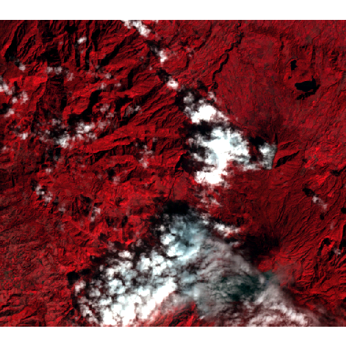
The fill image also has cloud cover, but less than the fill image - there are areas of the fill that can be used to fill clouded pixels in the base image:
plotRGB(fill, stretch='lin')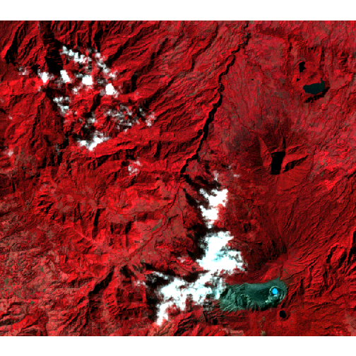
Topographic correction
In mountainous areas, topographic correction should be performed prior to cloud
fill1. teamlucc supports performing topographic correction using
algorithms derived from those in the landsat
package](http://cran.r-project.org/web/packages/landsat/index.html) by Sarah
Goslee3.
To perform topographic correction, use the topographic_corr function in
teamlucc. First load the slope and aspect rasters:
slp_asp <- brick('vb_slp_asp.tif')Now call the topographic_corr function twice, to topographically correct both
the base and fill image. Note that the sun angle elevation and sun azimuth
(both in degrees) must be supplied - values for these parameters can be found
in the metadata accompanying your imagery. See ?topographic_corr for more
information. DN_min and DN_max can be used to ensure that invalid values
are not generated by the topographic correction routine (which can sometimes be
a problem in very heavily shadowed areas, or in very bright areas, such as
clouds).
base_tc <- topographic_corr(base, slp_asp, sunelev=90-47.34, sunazimuth=134.04,
                            DN_min=0, DN_max=255)
## Warning: executing %dopar% sequentially: no parallel backend registeredfill_tc <- topographic_corr(fill, slp_asp, sunelev=90-46.80, sunazimuth=129.88,
DN_min=0, DN_max=255)plotRGB(base_tc, stretch='lin')
plotRGB(fill_tc, stretch='lin')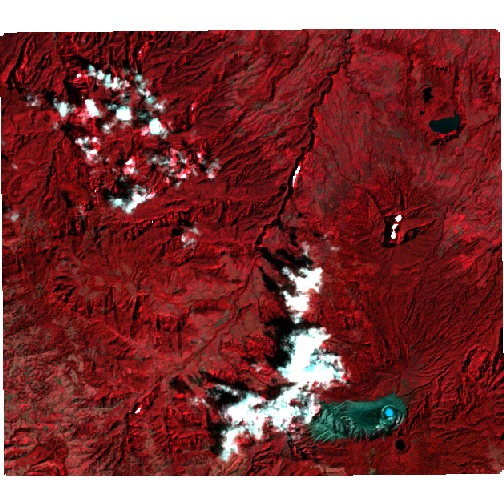
Construct cloud masks
The fmask band from the CDR imagery uses the following codes:
| Pixel type | Code |
|---|---|
| Clear land | 0 |
| Clear water | 1 |
| Cloud shadow | 2 |
| Snow | 3 |
| Cloud | 4 |
| No observation | 255 |
We need to construct a mask of areas where all pixels that are cloud (code 4)
or cloud shadow (code 2) are equal to 1, and where pixels in all other areas
are equal to zero. This is easy using raster algebra from the R raster
package. First load the masks:
base_fmask <- raster('vb_1986_005_fmask.tif')
fill_fmask <- raster('vb_1986_021_fmask.tif')
Now do the raster algebra, masking out clouds and cloud shadows, and setting missing values in both images to NAs in the masks:
# Set mask to 1 in clouds and shadow areas
base_cloud_mask <- (base_fmask == 2) | (base_fmask == 4)
fill_cloud_mask <- (fill_fmask == 2) | (fill_fmask == 4)
# Set mask to NA in background areas
base_cloud_mask[base_fmask == 255] <- NA
fill_cloud_mask[fill_fmask == 255] <- NA
# Set mask to NA in other NA areas in imagery (NAs can result from topographic
# correction, generally in very dark areas or areas of very high slope)
base_cloud_mask[is.na(base_tc[[1]])] <- NA
fill_cloud_mask[is.na(fill_tc[[1]])] <- NA
Plot these masks to double-check they align with the clouds in the images we viewed earlier:
plot(base_cloud_mask)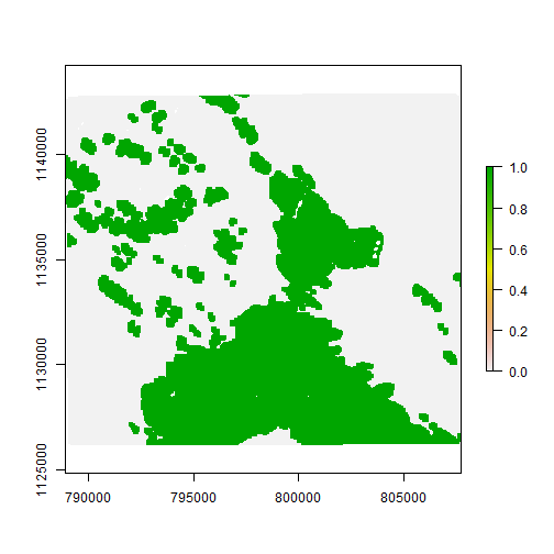
plot(fill_cloud_mask)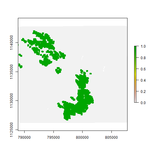
Now use these two masks to mask out the clouds in the fill and base images, by
setting clouded areas to zero (as the cloud_remove code treats pixels with
zero values as “background”:
base_tc[base_cloud_mask] <- 0
fill_tc[fill_cloud_mask] <- 0
The cloud mask for the base image must be constructed so that each cloud has
its own unique integer code, with codes starting from 1. This process can be
automated using the ConnCompLabel function from the SDMTools package.
However, because there are clouds in our fill image as well as in our base
image, we need to modify the base_cloud_mask slightly to account for this.
First, code all pixels in base_cloud_mask that are clouded in
fill_cloud_mask with NAs. This will tell the ConnCompLabel function not
to label these pixels as clouds (because they are also clouded in the fill
image, we cannot perform cloud fill on these pixels).
# Set clouds in fill image to NA in base mask:
base_cloud_mask[fill_cloud_mask] <- NA
# Set missing values in fill image to NA in base mask:
base_cloud_mask[is.na(fill_cloud_mask)] <- NA
Now run ConnCompLabel, and set the output datatype to INT2S (meaning the
data in base_cloud_mask can range from -32768 - 32767). That said, please
don’t try to run cloud fill with 32,767 clouds in your image :).
base_cloud_mask <- ConnCompLabel(base_cloud_mask)The final base_cloud_mask is now coded as:
| Pixel type | Code |
|---|---|
Background in fill or base |
NA |
Clouded in fill |
-1 |
Clear in base, clear in fill |
0 |
Clouded in base |
1 … n |
where n is the number of clouds in the image:
plot(base_cloud_mask)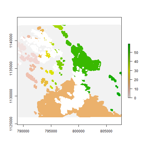
Fill clouds
For this simple example, we will directly use the cloud_remove function in
teamlucc. This function has a number of input parameters that can be supplied
(see ?cloud_remove). Two important ones to note are DN_min and DN_max.
These are the minimum and maximum valid values, respectively, that a pixel in
the image can take on. These limits are used to ignore unrealistic predictions
that may arise in the cloud fill routine. For the base and fill images we are
working with here, these values are 0 and 255, for max and min, respectively.
Set these parameters to appropriate values as necessary for the images you are
working with.
There are three different cloud fill algorithms that can be used from
teamlucc. Two require an IDL installation, while the third uses a cloud fill
algorithm that is native to R (though it is coded in C++ for speed reasons).
The R-based algorithm is a bit more flexible than the IDL algorithms, and is
designed to handle images in which both the base and fill image have clouds.
Based on the options supplied to cloud_remove, teamlucc will select one of
the fourt algorithms to run. The algorithm parameter to cloud_remove
determine which cloud fill algorithm is used:
| Algorithm | Requires IDL license? | Algorithm used by cloud_remove |
|---|---|---|
CLOUD_REMOVE |
Yes | CLOUD_REMOVE1 |
CLOUD_REMOVE_FAST |
Yes | CLOUD_REMOVE_FAST1 |
teamlucc |
No | teamlucc fill algorithm |
simple |
No | simple linear model algorithm |
First I will review the two IDL-based algorithms, then I will discuss the two R-based algorithms.
Cloud removal using IDL code
If run with algorithm="CLOUD_REMOVE" (the default), cloud_remove runs an
IDL script provided by Xiaolin Zhu. For
R to be able to run this script it must know the path to IDL on your machine.
For Windows users, this means the path to “idl.exe”. To specify this path you
will need to provide the idl parameter to the cloud_remove script. The
default value (C:/Program Files/Exelis/IDL83/bin/bin.x86_64/idl.exe) may or
may not work on your machine. I recommend you set the IDL path at the beginning
of your scripts:
idl_path <- "C:/Program Files/Exelis/IDL83/bin/bin.x86_64/idl.exe"An optional out_name parameter can be supplied to cloud_remove to specify
the filename for the output file. If not supplied, R will save the filled image
as an R object pointing to a temporary file.
To run the cloud removal routine, call the cloud_remove function with the
appropriate parameters. Note that this computation may take some time (it takes
around 1.5 hours on a 2.9Ghz Core-i7 3520M laptop).
# Takes 2-3 hours on a 2.9Ghz Core-i7 3520M laptop
start_time <- Sys.time()
# Ensure dataType is properly set prior to handing off to IDL
dataType(base_cloud_mask) <- 'INT2S'
filled_cr <- cloud_remove(base_tc, fill_tc, base_cloud_mask,
                            algorithm="CLOUD_REMOVE", DN_min=0, DN_max=255,
                            idl=idl_path)
## Loading required package: ncdfSys.time() - start_time## Time difference of 1.637638 hoursUse plotRGB to check the output. Note that IDL does not properly code missing
values in the output - prior to plotting or working with the data be sure to
set any pixels with values less than DN_min (here DN_min is zero) to NA:
filled_cr[filled_cr < 0] <- NA
plotRGB(filled_cr, stretch="lin")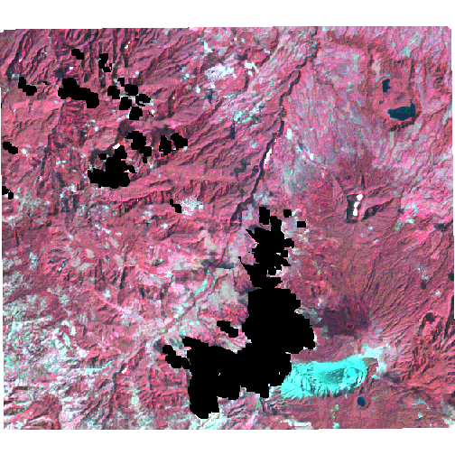
The default cloud fill approach can take a considerable amount of time to run.
There is an alternative approach that can take considerably less time to run,
with similar results. This option can be enabled by supplying the
algorithm="CLOUD_REMOVE_FAST parameter to cloud_remove.
The “fast” version of the algorithm makes some simplifications to improve
running time. Specifically, rather than follow the precise algorithm as
outlined by Zhu et al.1, the “fast” routine uses k-means clustering to
divide the image into the number of classes specified by the num_class
parameter. The script then constructs a linear model of the temporal change in
reflectance for each class within the neighborhood of a given cloud. This
“temporal” adjustment is complemented by a “spatial” adjustment that considers
the change in reflectance in a small neighborhood around each clouded pixel.
For each clouded pixel, a weighted combination of the predicted fill values
from the spatial and temporal models determines the final predicted value for
that pixel. This version of the algorithm takes only 2.5 minutes to run on the
same machine as used above:
# Takes 2-3 minutes on a 2.9Ghz Core-i7 3520M laptop
start_time <- Sys.time()
# Ensure dataType is properly set prior to handing off to IDL
dataType(base_cloud_mask) <- 'INT2S'
filled_crf  <- cloud_remove(base_tc, fill_tc, base_cloud_mask,
                                  algorithm="CLOUD_REMOVE_FAST", DN_min=0,
                                  DN_max=255, idl=idl_path)
Sys.time() - start_time
## Time difference of 55.48255 secsUse plotRGB to check the output:
filled_crf[filled_crf < 0] <- NA
plotRGB(filled_crf, stretch='lin')
Cloud removal using native R code
If you do not have IDL on your machine, there is a C++ implementation of the
NSPI cloud fill algorithm that will run directly in R, as well as a “simple”
cloud fill algorithm that uses linear models developed using the neighborhood
of each cloud to perform a naive fill. To run the R version of the NSPI
algorithm, call the cloud_remove function with the same parameters as above,
but specify algorithm="teamlucc". This function also has a verbose=TRUE
option to tell cloud_remove to print progress statements as it is running
(this option is not available with the IDL scripts shown above). This version
is nearly identical to the IDL algorithm called with the
algorithm="CLOUD_REMOVE" option, but it takes much less time to run (only 3-4 minutes on my machine).
Note that when cloud_remove is run with algorithm="teamlucc" and
verbose=TRUE, there will be a large number of status messages printed to the
screen. For the purposes of this demo (so that the webpage is not unnecessarily
long), I have not used the verbose=TRUE argument, but I recommend using it if
you try this command yourself.
# Takes 4-5 minutes on a 2.9Ghz Core-i7 3520M laptop
start_time <- Sys.time()
filled_tl <- cloud_remove(base_tc, fill_tc, base_cloud_mask, DN_min=0,
                              DN_max=255, algorithm="teamlucc")
Sys.time() - start_time
## Time difference of 3.320532 minsView the results with plotRGB:
plotRGB(filled_tl, stretch='lin')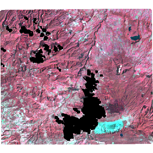
The fastest cloud fill option is to run cloud_remove with
algorithm="SIMPLE". This uses a simple cloud fill approach in which the value
of each clouded pixel is calculated using a linear model. The script develops a
separate linear model (with slope and intercept) for each band and each cloud.
For each cloud, and each image band, the script finds all pixels clear in both
the cloudy and fill images, and calculates a regression model in which pixel
values in the fill image are the independent variable, and pixel values in the
clouded image are the dependent variable. The script then uses this model to
predict pixel values for each band in each cloud in the clouded image. For
example:
# Takes 2-5 seconds on a 2.9Ghz Core-i7 3520M laptop
start_time <- Sys.time()
filled_simple <- cloud_remove(base_tc, fill_tc, base_cloud_mask, DN_min=0,
                              DN_max=255, algorithm="simple")
Sys.time() - start_time
## Time difference of 0.6300631 secsView the results with plotRGB:
plotRGB(filled_simple, stretch='lin')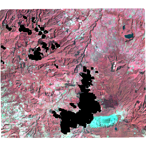
Compare all four fill algorithms:
To plot the results of all four fill algorithms, make a layer stack of the first band of all four images, then plot:
filled_comp <- stack(filled_cr[[1]], filled_crf[[1]], filled_tl[[1]],
                     filled_simple[[1]])
names(filled_comp) <- c('CLOUD_REMOVE', 'CLOUD_REMOVE_FAST', 'teamlucc',
                       'simple')
filled_comp <- linear_stretch(filled_comp, pct=2, max_val=255)
plot(filled_comp)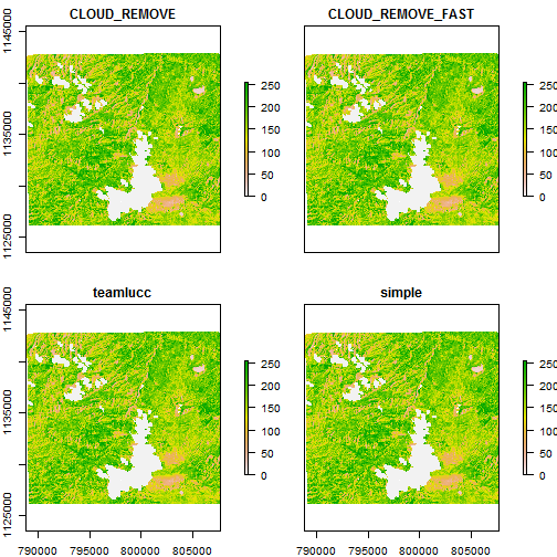
Automated cloud fill from an image time series
The teamlucc package also includes functions for automated cloud filling from
an image time series. Automatic cloud filling is performed using the
auto_cloud_fill function. This function automates the majority of the cloud
filling process. As multiple images are required to demonstrate this process,
the images required for this portion of the example are not available for
download from this site. I suggest you download the appropriate imagery for a
particular study site and preprocess the imagery using the auto_setup_dem and
auto_preprocess_landsat functions in the teamlucc package so that you can
follow along with this example. The auto_preprocess_landsat function will
also perform topographic correction, which is necessary prior to cloud filling
images in mountainous areas.
The auto_cloud_fill function allows an analyst to automatically construct a
cloud-filled image after specifying: data_dir (a folder of Landsat
images), wrspath and wrsrow (the WRS-2 path/row to use), and start_date
and end_date (a start and end date limiting the images to use in the
algorithm). The analyst can also optionally specify a base_date, and the
auto_cloud_fill function will automatically pick the image closest to that
date to use as the base image (otherwise auto_cloud_fill will automatically
pick the image with the least cloud cover as the base image).
As the auto_cloud_fill function automatically chooses images for inclusion in
the cloud fill process, it relies on having images stored on disk in a
particular way, and currently only supports cloud fill for Landsat CDR surface
reflectance images. To ensure that images are correctly stored on your hard
disk, use the auto_preprocess_landsat function to extract the original
Landsat CDR hdf files from the USGS archive. The auto_preprocess_landsat
function will ensure that images are extracted and renamed properly so that
they can be used with the auto_cloud_fill script.
# start_time <- Sys.time()
# start_date <- as.Date('1986-01-01')
# end_date <- as.Date('1987-01-01')
# filled_image <- auto_cloud_fill("C:/Data/LEDAPS_imagery", wrspath=230,
#                                 wrsrow=62, start_date=start_date,
#                                 end_date=end_date)
# Sys.time() - start_time-
Zhu, X., Gao, F., Liu, D., Chen, J., 2012. A modified neighborhood similar pixel interpolator approach for removing thick clouds in Landsat images. Geoscience and Remote Sensing Letters, IEEE 9, 521–525. doi:10.1109/LGRS.2011.2173290 ↩ ↩2 ↩3 ↩4 ↩5
-
Zhu, Z. and Woodcock, C. E., Object-based cloud and cloud shadow detection in Landsat imagery, Remote Sensing of Environment (2012), doi:10.1016/j.rse.2011.10.028 ↩
-
Sarah C. Goslee (2011). Analyzing Remote Sensing Data in R: The landsat Package. Journal of Statistical Software, 43(4), 1-25. ↩
