This post outlines how to use the glcm package to calculate image textures that are direction invariant (calculated over “all directions”). This feature is only available in glcm versions >= 1.0.

Getting started

First use install the latest version of glcm, and the raster package that is also needed for this example:

install.packages("glcm")

## Installing package into 'C:/Users/azvoleff/R/win-library/3.1'
## (as 'lib' is unspecified)

## package 'glcm' successfully unpacked and MD5 sums checked
## 
## The downloaded binary packages are in
## 	C:\Users\azvoleff\AppData\Local\Temp\Rtmp2j8wNL\downloaded_packages

library(glcm)
library(raster)

## Loading required package: sp

Calculating rotationally invariant textures

glcm supports calculating GLCMs using multiple shift values. If multiple shifts are supplied, glcm will calculate each texture statistic using each of the specified shifts, and return the mean value of the texture for each pixel.
In general, I have not found large differences in calculated image textures when comparing GLCM textures calculated using a single shift versus calculating rotationally invariant textures. However this may not be the case for images with strongly directional textures.

To compare for a sample cropped out of a Landsat scene, use the L5TSR_1986 sample image included in the glcm package. This is a section of a 1986 Landsat 5 image preprocessed to surface reflectance. The image is from the Volcán Barva TEAM site.

When glcm is run without specifing a shift, the default shift (1, 1) is used (90 degrees), with a window size of 3 pixels x 3 pixels. Below is an example from running glcm with the default parameters:

test_rast <- raster(L5TSR_1986, layer=1)
tex_shift1 <- glcm(test_rast)
plot(tex_shift1)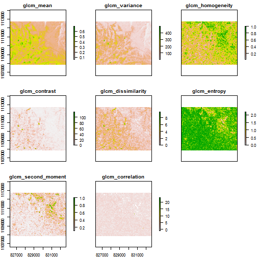

To calculate rotationally invariant GLCM textures (over “all directions” in the terminology of commonly used remote sensing software), use: shift=list(c(0,1), c(1,1), c(1,0), c(1,-1)). This will calculate the average GLCM texture using shifts of 0 degrees, 45 degrees, 90 degrees, and 135 degrees:

tex_all_dir <- glcm(test_rast, shift=list(c(0,1), c(1,1), c(1,0), c(1,-1)))
plot(tex_all_dir)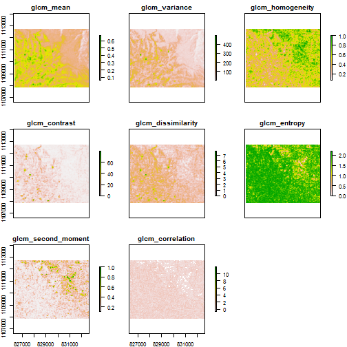

To compare the difference between these textures, subtract the textures calculated with a 90 degree shift from those calculated using multiple shifts, and plot the result:

plot((tex_all_dir - tex_shift1) / tex_all_dir)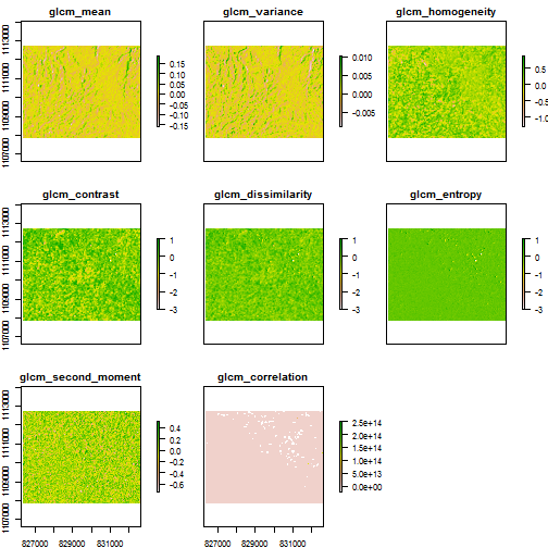

Computation time

First look at the time difference for calculating a GLCM with only one shift versus calculating a rotationally invariant form:

library(microbenchmark)

glcm_one_dir <- function(x) {
    glcm(x)
}

glcm_all_dir <- function(x) {
    glcm(x, shift=list(c(0,1), c(1,1), c(1,0), c(1,-1)))
}

microbenchmark(glcm_one_dir(test_rast), glcm_all_dir(test_rast), times=5)

## Unit: seconds
##                     expr      min       lq     mean   median       uq
##  glcm_one_dir(test_rast) 1.090759 1.117674 1.141704 1.146656 1.154196
##  glcm_all_dir(test_rast) 4.090347 4.108833 4.189145 4.116991 4.164241
##       max neval
##  1.199236     5
##  4.465313     5

As seen in the above, there is a performance penalty for using a rotationally invariant GLCM (not surprisingly, as more calculations are involved).

Prior to having the ability to use multiple shifts hardcoded in glcm, it was still possible to calculate rotationally invariant textures using the glcm function. However, the calculation had to be done manually, using an approach similar to what I do below with glcm_all_dir_manual. How much faster is it perform the averaging directly in glcm?

glcm_all_dir_manual <- function(x) {
    text_0deg <- glcm(x, shift=c(0,1))
    text_45deg <- glcm(x, shift=c(1,1))
    text_90deg <- glcm(x, shift=c(1,0))
    text_135deg <- glcm(x, shift=c(1,-1))
    overlay(text_0deg, text_45deg, text_90deg, text_135deg,
            fun=function(w, x, y, z) {
                return((w + x + y + z) / 4)
            })
}
tex_all_dir_manual <- glcm_all_dir_manual(test_rast)

# Check that the textures match
table(getValues(tex_all_dir_manual) == getValues(tex_all_dir))

## 
##   TRUE 
## 273488

microbenchmark(glcm_all_dir_manual(test_rast), glcm_all_dir(test_rast), 
               times=5)

## Unit: seconds
##                            expr      min       lq     mean   median
##  glcm_all_dir_manual(test_rast) 4.493543 4.501502 4.678655 4.656803
##         glcm_all_dir(test_rast) 4.134398 4.190528 4.267464 4.225021
##        uq      max neval
##  4.809615 4.931815     5
##  4.304919 4.482455     5

The time difference isn’t that great, but the need for repeated calls to glcm (and the need for multiple read/writes to disk for large files) could lead to a more substantial advantage for the direct approach with glcm than is apparent in this simple example. Of course, the manual approach does give more flexibility if you need to do other processing (or scaling, etc.) to the textures.