Getting started

First load the devtools package, used for installing teamlucc. Install the devtools package if it is not already installed:

if (!require(devtools)) {
    install.packages('devtools')
    library(devtools)
}

Now load the teamlucc package, using devtools to install it from github if it is not yet installed:

if (!require(teamlucc)) {
    install_github('azvoleff/teamlucc')
    library(teamlucc)
}

Also load the rgdal package needed for reading/writing shapefiles:

library(rgdal)

## rgdal: version: 0.9-1, (SVN revision 518)
## Geospatial Data Abstraction Library extensions to R successfully loaded
## Loaded GDAL runtime: GDAL 1.11.0, released 2014/04/16
## Path to GDAL shared files: C:/Users/azvoleff/R/win-library/3.1/rgdal/gdal
## GDAL does not use iconv for recoding strings.
## Loaded PROJ.4 runtime: Rel. 4.8.0, 6 March 2012, [PJ_VERSION: 480]
## Path to PROJ.4 shared files: C:/Users/azvoleff/R/win-library/3.1/rgdal/proj

Collect training data for supervised classification

The first step in the classification is putting together a training dataset. teamlucc includes a function to output a shapefile that can be used for collecting training data. Here we are collecting training data for the L5TSR_1986 raster (a portion of a 1986 Landsat 5 surface reflectance image) that is included with the teamlucc package. Use the get_extent_polys function to quickly construct a shapefile in the same coordinate system as the image:

train_polys <- get_extent_polys(L5TSR_1986)

Add an empty field named “class_1986” to the object, and delete the extent polygon (because we don’t need it, and just want an empty shapefile):

train_polys$class_1986 <- '' # Add an empty column named "class_1986"
train_polys <- train_polys[-1, ] # Delete extent polygon

Now save the train_polys object to a shapefile using writeOGR from the rgdal package. The "." below just means “save the shapefile in the current directory”.

writeOGR(train_polys, ".", "training_data", "ESRI Shapefile")

Open the generated “training_data.shp” shapefile in a GIS program (I recommend QGIS) and digitize a number of polygons in each of the land cover classes you want to map. For this example, we will simply classify “Forest” and “Non-forest”. For each polygon you digitize, record the cover type in the “class_1986” column. After digitizing a number of polygons within each class, save the shapefile, and load it back into R using train_polys <- readOGR(".", "training_data").

Or: (for this example) you can use the thirty training polygons included in the teamlucc package in the L5TSR_1986_2001_training dataset:

train_polys <- L5TSR_1986_2001_training

Classify image

First we need to extract the training data from our training image, for each pixel within the polygons in our train_polys dataset. get_pixels will use the training parameter that we pass to determine the fraction of the training data to use in training the classifier. If set to 1, ALL of the training data will be used to train the classifier, leaving no independent data for validation. If set to a fraction (for example .6), then only 60% of the data (randomly selected) will be used in training, and 40% will be preserved as an independent sample for use in testing.

Note: Validation data should generally be collected separately from training data anyways, to ensure the image is randomly sampled (training data collection is almost never random), so in most cases I don’t recommend making heavy use of the training parameter. It can be useful though in testing.

set.seed(0) # Set a random seed so results can be reproduced
train_data <- get_pixels(L5TSR_1986, train_polys, class_col="class_1986", 
                         training=.6)

A summary method is provided by teamlucc for printing summary statistics on training datasets:

summary(train_data)

## Object of class "pixel_data"
## 
## Number of classes:	2
## Number of polygons:	30
## Number of pixels:	120
## Number of sources:	1
## 
## Training data statistics:
## Source: local data frame [2 x 5]
## 
##       class n_polys n_train_pixels n_test_pixels train_frac
## 1    Forest      17             48            20       0.71
## 2 NonForest      13             24            28       0.46
## 
## Number of training samples:	72
## Number of testing samples:	48
## Training fraction:		0.6

To perform the actual image classification, we will use the classify function. Prior to using that function, we need to train a classifier. The train_classifier function automates training a random forest or support vector machine (SVM) classifier. There are many options that can be provided to train_classifier - for this example we will just use the defaults. The default is to use a random forest classifier.

clfr <- train_classifier(train_data)

## Loading required package: randomForest
## randomForest 4.6-10
## Type rfNews() to see new features/changes/bug fixes.
## Loading required package: lattice
## Loading required package: ggplot2

Now we can use the classify function to perform the image classification:

cls <- classify(L5TSR_1986, clfr)

## Warning in .local(x, ...): min value not known, use setMinMax

## Warning in .local(x, ...): min value not known, use setMinMax

## Loading required package: parallel
## 
## Attaching package: 'parallel'
## 
## The following objects are masked from 'package:snow':
## 
##     clusterApply, clusterApplyLB, clusterCall, clusterEvalQ,
##     clusterExport, clusterMap, clusterSplit, makeCluster,
##     parApply, parCapply, parLapply, parRapply, parSapply,
##     splitIndices, stopCluster
## 
## Loading required package: iterators
## Loading required package: foreach
## foreach: simple, scalable parallel programming from Revolution Analytics
## Use Revolution R for scalability, fault tolerance and more.
## http://www.revolutionanalytics.com
## 
## Attaching package: 'mmap'
## 
## The following object is masked from 'package:Rcpp':
## 
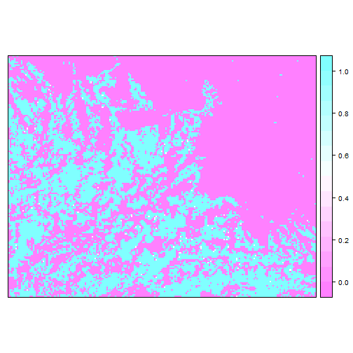
##     sizeof

## Warning in int64(): unsupported int64, use int32 or real64

To see the predicted classes, use spplot:

spplot(cls$classes)

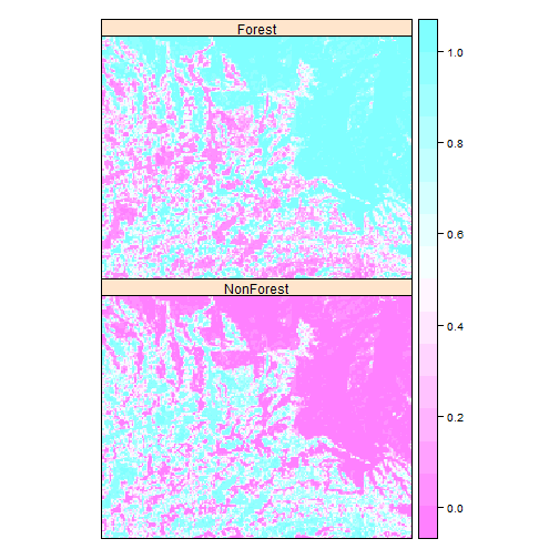
We can also see the class probabilities (per pixel probabilities of membership of each class):

spplot(cls$probs)

The output from classify also includes a table indicating the coding for the output:

print(cls$codes)

##   code     class
## 1    0    Forest
## 2    1 NonForest

Parallel processing

Training a classifier and predicting land cover classes is very CPU-intensive.
If you have a machine that has multiple processors (or multiple cores), using more than one processor can significantly increase the speed of some calculations. teamlucc supports parallel computations (using the capabilities of the raster package). To enable this functionality, first install the doParallel package if it is not already installed, and load the package:

if (!require(doParallel)) {
    install.packages('doParallel')
    library(doParallel)
}

## Loading required package: doParallel

Now, just call registerDoParallel(), and by default any calculations that are coded to run in parallel will use half of the available CPUs on your machine.
You can also specify a number of CPUs to use, by running, for example, registerDoParallel(2) to use two CPUs. The get_pixels, train_classifier
and classify functions in teamlucc all support parallel computation, and will run in parallel automatically if you have called registerDoParallel.
Below is the code for the same classification problem we just ran, but this time we run the classification in parallel:

library(doParallel)
registerDoParallel(2)
set.seed(0) # Set a random seed so results match what we got earlier
train_data_par <- get_pixels(L5TSR_1986, train_polys, class_col="class_1986", 
                             training=.6)
clfr_par <- train_classifier(train_data)
cls_par <- classify(L5TSR_1986, clfr)

## Warning in .local(x, ...): min value not known, use setMinMax

## Warning in .local(x, ...): min value not known, use setMinMax

Accuracy assessment

Conducting a thorough accuracy assessment is one of the most important components of image classification. The teamlucc package includes an accuracy function to assist with measuring the accuracy of image classifications. In addition to the standard contingency tables often used for describing accuracy, accuracy also calculates “quantity disagreement” and “allocation disagreement” as introduced by Pontius and Millones 2011¹.
Unbiased contingency tables can be calculated with accuracy by supplying a pop parameter to accuracy. accuracy provides 95% confidence intervals for user’s, producer’s, and overall accuracies, calculated as in Olofsson et al.
2013².

To calculate a basic contingency table, assuming that population frequencies of the observed classes can be estimated from the classification output, and using the 40% of pixels that were excluded from training the classifier as testing data, run the accuracy function using the model calculated above:

acc <- accuracy(clfr)

## Warning in calc_accuracy(predicted, observed, pop, reclass_mat): pop was
## not provided - assuming sample frequencies equal population frequencies

Note the warning from accuracy, which is reminding us that we did not provide population frequencies for the classes.

Asummary method for the accuracy object is provided by teamlucc, and calculates user’s, producers, and overall accuracy, and quantity and allocation disagreement:

summary(acc)

## Object of class "accuracy"
## 
## Testing samples:	48
## 
## Sample contingency table:
##            observed
## predicted    Forest NonForest   Total   Users
##   Forest    16.0000    3.0000 19.0000  0.8421
##   NonForest  4.0000   25.0000 29.0000  0.8621
##   Total     20.0000   28.0000 48.0000        
##   Producers  0.8000    0.8929          0.8542
## 
## Population contingency table:
##            observed
## predicted   Forest NonForest  Total  Users
##   Forest    0.3333    0.0625 0.3958 0.8421
##   NonForest 0.0833    0.5208 0.6042 0.8621
##   Total     0.4167    0.5833 1.0000       
##   Producers 0.8000    0.8929        0.8542
## 
## Overall accuracy:	0.8542
## 
## Quantity disagreement:		0.0208
## Allocation disagreement:	0.125