Analyzing forest change with gfcanalysis
Overview
The gfcanalysis R package facilitates simple analyses using the Hansen et al. 2013 Global Forest Change dataset. The package was written to analyze forest change within the Zone of Interaction surrounding each of the forest monitoring sites of the Tropical Ecology Assessment and Monitoring (TEAM) Network.
Hansen, M. C., P. V. Potapov, R. Moore, M. Hancher, S. A. Turubanova, A. Tyukavina, D. Thau, S. V. Stehman, S. J. Goetz, T. R. Loveland, A. Kommareddy, A. Egorov, L. Chini, C. O. Justice, and J. R. G. Townshend. 2013. High-Resolution Global Maps of 21st-Century Forest Cover Change. Science 342, (15 November): 850-853.
If you need help with any of the functions in the package, see the help files for more information. For example, type ?download_tiles in R to see the help file for the download_tiles function.
Getting started
This post will outline an analysis using the gfcanalysis package. Note that as the computations are intensive, some parts of this analysis may take some time to run. If you do not already have the GFC product data downloaded on your computer, downloading the dataset will also take some time (though this process is automated by gfcanalysis).
To get started, first install the gfcanalysis package from CRAN:
if (!require(gfcanalysis)) install.packages('gfcanalysis')
if (!require(rgdal)) install.packages('rgdal')
Indicate where we want to save GFC tiles downloaded from Google. For any given AOI, the script will first check to see if these tiles are available locally before downloading them from the server:
output_folder <- "."Set the threshold for forest/non-forest based on the treecover2000 layer in the GFC product:
forest_threshold <- 90Downloading data from Google server for a given AOI
Load an area of interest. For this example we use a shapefile of the Zone of Interaction (ZOI) of the TEAM Network site in Nam Kading National Protected Area, Laos.
You can download the shapefile of the ZOI to follow along with this example.
aoi <- readOGR('.', 'ZOI_NAK_2012_EEsimple')Calculate the tiles needed to cover the AOI:
tiles <- calc_gfc_tiles(aoi)
print(length(tiles)) # Number of tiles needed to cover AOI
## [1] 1
To check the overlap between the tiles and the AOI, you can make a plot:
plot(tiles)
plot(aoi, add=TRUE, lty=2, col="#00ff0050")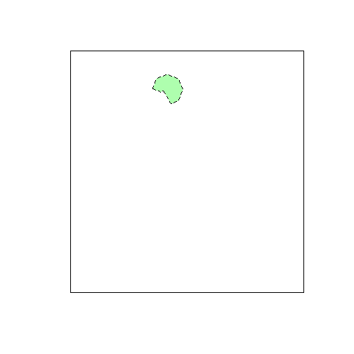
Now, check to see if these tiles are already present locally, and download them if they are not:
download_tiles(tiles, output_folder, first_and_last=FALSE)
## 1 tiles to download/check.
## 0 file(s) succeeded, 5 file(s) skipped, 0 file(s) failed.
Performing thresholding and calculating basic statistics
Extract the GFC data for this AOI from the downloaded GFC tiles, mosaicing multiple tiles as necessary:
gfc_extract <- extract_gfc(aoi, output_folder, filename="NAK_GFC_extract.tif")The extracted dataset has 5 layers (not yet thresholded):
- treecover2000
- loss
- gain
- lossyear
- datamask
Threshold the GFC data based on the specified percent cover threshold:
gfc_thresholded <- threshold_gfc(gfc_extract, forest_threshold=forest_threshold,
                                 filename="NAK_GFC_extract_thresholded.tif")
Coding of the thresholded output
Band 1 (forest2000)
| Value | Meaning |
|---|---|
| 0 | Non-forest |
| 1 | Forest |
Band 2 (lossyear)
| Value | Meaning |
|---|---|
| 0 | No loss |
| 1-12 | Loss in 2001-2012 |
Band 3 (gain)
| Value | Meaning |
|---|---|
| 0 | No gain |
| 1 | Gain |
Band 4 (lossgain)
| Value | Meaning |
|---|---|
| 0 | No loss and gain |
| 1 | Loss and gain |
Band 5 (datamask)
| Value | Meaning |
|---|---|
| 0 | No data |
| 1 | Land |
| 2 | Water |
Calculating statistics on forest loss and forest gain
Calculate annual statistics on forest loss/gain:
gfc_stats <- gfc_stats(aoi, gfc_thresholded)
gfc_stats
Save these statistics to CSV files:
write.csv(gfc_stats$loss_table,
          file='NAK_GFC_extract_thresholded_losstable.csv', row.names=FALSE)
write.csv(gfc_stats$gain_table,
          file='NAK_GFC_extract_thresholded_gaintable.csv', row.names=FALSE)
View the sample output files:
Making simple visualizations
There is also a function to calculate and save a thresholded annual layer stack:
gfc_annual_stack <- annual_stack(gfc_thresholded)
writeRaster(gfc_annual_stack, filename="NAK_GFC_extract_thresholded_annual.tif")
Forest change in each year is coded as:
| Value | Meaning |
|---|---|
| 0 | No data |
| 1 | Forest |
| 2 | Non-forest |
| 3 | Forest loss |
| 4 | Forest gain |
| 5 | Forest loss and gain |
| 6 | Water |
The animate_annual function can be used to save a simple visualization of the thresholded annual layer stack:
aoi$label <- "ZOI" # Label the polygon on the plot
animate_annual(aoi, gfc_annual_stack, out_dir='.', site_name='Nam Kading')
View the animation for Nam Kading.
Learn More
The full documentation for the gfcanalysis package is available on CRAN.